Blinda's Class
Classwork for BIMM143
Lab 07 Machine Learning 1
Blinda Sui (PID: A17117043)
Today we will explore some fundamental machine learning methods including clustering and dimensionality reduction.
K-means clustering
To see how this works let’s first makeup some data to cluster where we
know what the answer should be. We can use the rnorm() function to
help here:
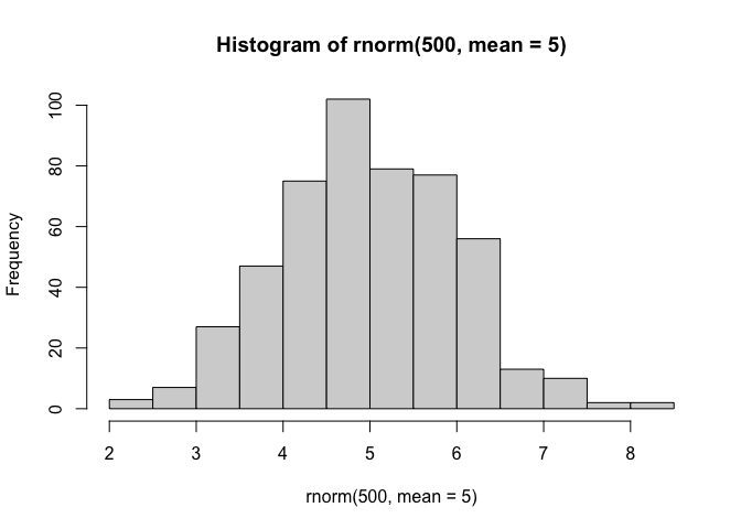
hist(rnorm(500, mean=5))
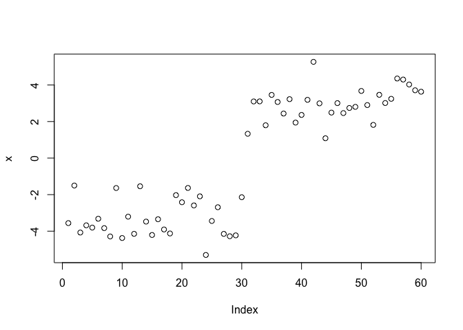
x <- c(rnorm(30, mean=-3),rnorm(30, mean=3))
y <- rev(x) #reverse x
cbind(x, y)
              x         y
 [1,] -3.558170  3.632061
 [2,] -1.501385  3.710897
 [3,] -4.074267  4.027479
 [4,] -3.679126  4.299014
 [5,] -3.804401  4.355379
 [6,] -3.319883  3.243559
 [7,] -3.832704  3.013477
 [8,] -4.289685  3.463544
 [9,] -1.637985  1.816822
[10,] -4.374156  2.901404
[11,] -3.204849  3.673818
[12,] -4.145656  2.803598
[13,] -1.541535  2.742934
[14,] -3.476352  2.463249
[15,] -4.208345  3.008345
[16,] -3.346022  2.490190
[17,] -3.906891  1.085147
[18,] -4.125254  2.995049
[19,] -2.027630  5.267389
[20,] -2.417331  3.188682
[21,] -1.634382  2.361781
[22,] -2.590232  1.942936
[23,] -2.093131  3.225211
[24,] -5.301714  2.437554
[25,] -3.442146  3.071399
[26,] -2.689639  3.458139
[27,] -4.147775  1.796105
[28,] -4.277262  3.103786
[29,] -4.229445  3.100339
[30,] -2.141675  1.330859
[31,]  1.330859 -2.141675
[32,]  3.100339 -4.229445
[33,]  3.103786 -4.277262
[34,]  1.796105 -4.147775
[35,]  3.458139 -2.689639
[36,]  3.071399 -3.442146
[37,]  2.437554 -5.301714
[38,]  3.225211 -2.093131
[39,]  1.942936 -2.590232
[40,]  2.361781 -1.634382
[41,]  3.188682 -2.417331
[42,]  5.267389 -2.027630
[43,]  2.995049 -4.125254
[44,]  1.085147 -3.906891
[45,]  2.490190 -3.346022
[46,]  3.008345 -4.208345
[47,]  2.463249 -3.476352
[48,]  2.742934 -1.541535
[49,]  2.803598 -4.145656
[50,]  3.673818 -3.204849
[51,]  2.901404 -4.374156
[52,]  1.816822 -1.637985
[53,]  3.463544 -4.289685
[54,]  3.013477 -3.832704
[55,]  3.243559 -3.319883
[56,]  4.355379 -3.804401
[57,]  4.299014 -3.679126
[58,]  4.027479 -4.074267
[59,]  3.710897 -1.501385
[60,]  3.632061 -3.558170
plot(x)
The function for K-means clustering in “base” R is kmeans()
kmeans(x, centers = 2)
K-means clustering with 2 clusters of sizes 30, 30

Cluster means:
       [,1]
1  3.000338
2 -3.300634

Clustering vector:
 [1] 2 2 2 2 2 2 2 2 2 2 2 2 2 2 2 2 2 2 2 2 2 2 2 2 2 2 2 2 2 2 1 1 1 1 1 1 1 1
[39] 1 1 1 1 1 1 1 1 1 1 1 1 1 1 1 1 1 1 1 1 1 1

Within cluster sum of squares by cluster:
[1] 23.48218 30.61468
 (between_SS / total_SS =  91.7 %)

Available components:

[1] "cluster"      "centers"      "totss"        "withinss"     "tot.withinss"
[6] "betweenss"    "size"         "iter"         "ifault"
k <- kmeans(x, centers = 2)
k
K-means clustering with 2 clusters of sizes 30, 30

Cluster means:
       [,1]
1  3.000338
2 -3.300634

Clustering vector:
 [1] 2 2 2 2 2 2 2 2 2 2 2 2 2 2 2 2 2 2 2 2 2 2 2 2 2 2 2 2 2 2 1 1 1 1 1 1 1 1
[39] 1 1 1 1 1 1 1 1 1 1 1 1 1 1 1 1 1 1 1 1 1 1

Within cluster sum of squares by cluster:
[1] 23.48218 30.61468
 (between_SS / total_SS =  91.7 %)

Available components:

[1] "cluster"      "centers"      "totss"        "withinss"     "tot.withinss"
[6] "betweenss"    "size"         "iter"         "ifault"
#:) Clustering vector: the first 30 belongs to cluster 1 and last 30 belongs to cluster 2 #:) Within cluster sume of squares by cluster (WCSS): For k=2 clusters, these are the WCSS values for cluster 1 and cluster 2. Lower = tighter cluster. Here, cluster 2 is looser (30.12 > 16.66). #:) (between_SS / total_SS = 92.4%): the proportion of total variance “explained” by the separation between the two cluster centroids = only 7.6% of the variance remains within clusters.
To get the results of the returned list object we can use the dollar $
syntax.
Q. How many points are in each cluster?
k$size
[1] 30 30
Q. What ‘component’ of your result object details - cluster assignment/membership? - cluster center?
k$cluster
 [1] 2 2 2 2 2 2 2 2 2 2 2 2 2 2 2 2 2 2 2 2 2 2 2 2 2 2 2 2 2 2 1 1 1 1 1 1 1 1
[39] 1 1 1 1 1 1 1 1 1 1 1 1 1 1 1 1 1 1 1 1 1 1
k$centers
       [,1]
1  3.000338
2 -3.300634
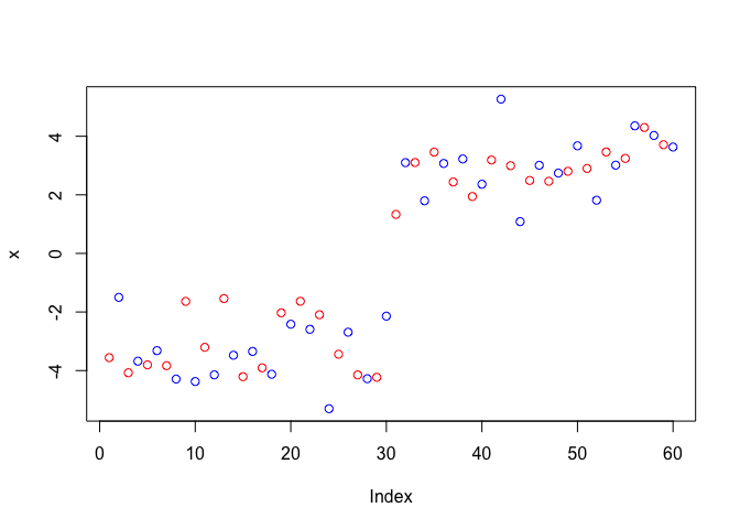
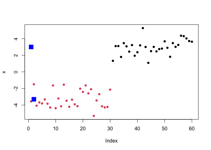
Q. Make a clustering results figure of the data colored by cluster membership and show cluster centers.
plot(x, col = c("red", "blue"))
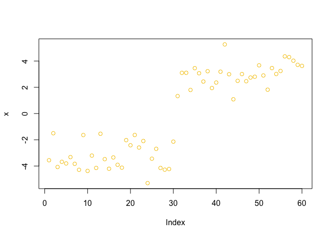
plot(x, col = 7)
plot(x, col = k$cluster, pch=16)
points(k$centers, col="blue", pch=15, cex=2)
K-means clustering is very popular as it is very fast and relatively straight forward: it takes numeric data as input and returns the clusterm membership vector etc.
The “issue” is we tell kmeans() how many clusters we want!
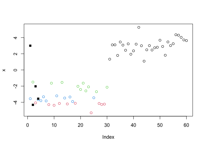
Q. Run kmeans again and cluster into 4 frps/clusters and plot the results like we did above?
k4 <- kmeans(x, centers = 4)
plot(x, col=k4$cluster)
points(k4$centers, pch=15)
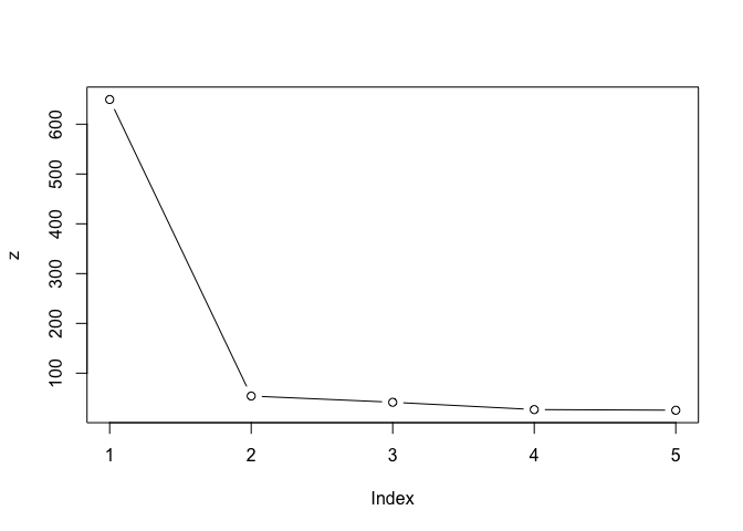
Scree plot to pick k center value
brute-force
k1 <- kmeans(x, centers = 1)
k2 <- kmeans(x, centers = 2)
k3 <- kmeans(x, centers = 3)
k4 <- kmeans(x, centers = 4)
k5 <- kmeans(x, centers = 5)
z <- c(k1$tot.withinss,
       k2$tot.withinss,
       k3$tot.withinss,
       k4$tot.withinss,
       k5$tot.withinss)

plot(z, typ = "b")
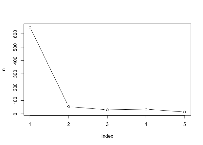
n <- NULL
for(i in 1:5) {
  n <- c(n, kmeans(x, centers = i)$tot.withinss)
}

plot(n, typ = "b")
Hierarchical CLustering
The main “base” R function for Hierarchical Clustering is called
cluster(). Here we can’t just input our data, we need to first
calculate a distance matrix (e.g.dist()) for our data and use this as
input to hclust()
d <- dist(x)
hc <- hclust(d)
hc
Call:
hclust(d = d)

Cluster method   : complete
Distance         : euclidean
Number of objects: 60
There is a plot method for hclust results, lets try it
plot(hc)
abline(h=8, col="red") #abline(): to add straight lines to an existing plot.
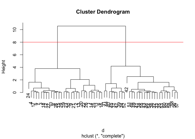
To get our cluster “membership” vector (i.e. our main clustering result) we can “cut” the tree at a given height or at height that yields a given “k” gorups.
cutree(hc, h=8)
 [1] 1 1 1 1 1 1 1 1 1 1 1 1 1 1 1 1 1 1 1 1 1 1 1 1 1 1 1 1 1 1 2 2 2 2 2 2 2 2
[39] 2 2 2 2 2 2 2 2 2 2 2 2 2 2 2 2 2 2 2 2 2 2
grps <- cutree(hc, k=2)
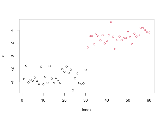
Q. Plot the data with our hclust result coloring
plot(x, col=grps)
Principal Component Analysis (PCA)
PCA of UK food data
Import food data from an online CSV file:
url <- "https://tinyurl.com/UK-foods"
x <- read.csv(url)
head(x)
               X England Wales Scotland N.Ireland
1         Cheese     105   103      103        66
2  Carcass_meat      245   227      242       267
3    Other_meat      685   803      750       586
4           Fish     147   160      122        93
5 Fats_and_oils      193   235      184       209
6         Sugars     156   175      147       139
rownames(x) <- x[, 1]
x <- x[, -1]
x
                    England Wales Scotland N.Ireland
Cheese                  105   103      103        66
Carcass_meat            245   227      242       267
Other_meat              685   803      750       586
Fish                    147   160      122        93
Fats_and_oils           193   235      184       209
Sugars                  156   175      147       139
Fresh_potatoes          720   874      566      1033
Fresh_Veg               253   265      171       143
Other_Veg               488   570      418       355
Processed_potatoes      198   203      220       187
Processed_Veg           360   365      337       334
Fresh_fruit            1102  1137      957       674
Cereals                1472  1582     1462      1494
Beverages                57    73       53        47
Soft_drinks            1374  1256     1572      1506
Alcoholic_drinks        375   475      458       135
Confectionery            54    64       62        41
x <- read.csv(url, row.names = 1)
x
                    England Wales Scotland N.Ireland
Cheese                  105   103      103        66
Carcass_meat            245   227      242       267
Other_meat              685   803      750       586
Fish                    147   160      122        93
Fats_and_oils           193   235      184       209
Sugars                  156   175      147       139
Fresh_potatoes          720   874      566      1033
Fresh_Veg               253   265      171       143
Other_Veg               488   570      418       355
Processed_potatoes      198   203      220       187
Processed_Veg           360   365      337       334
Fresh_fruit            1102  1137      957       674
Cereals                1472  1582     1462      1494
Beverages                57    73       53        47
Soft_drinks            1374  1256     1572      1506
Alcoholic_drinks        375   475      458       135
Confectionery            54    64       62        41
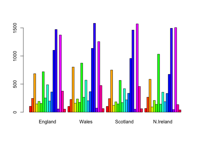
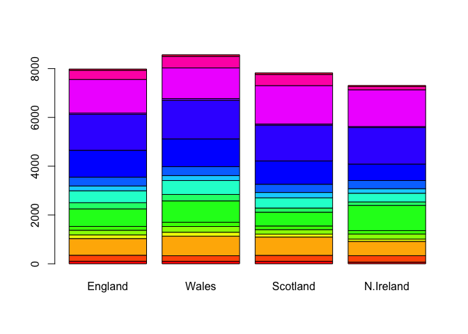
some base figures
barplot(as.matrix(x), beside=T, col=rainbow(nrow(x)))
barplot(as.matrix(x), beside=F, col=rainbow(nrow(x)))
There is one plot that can be useful for small datasets:
pairs(x, col=rainbow(nrow(x)), pch=16)
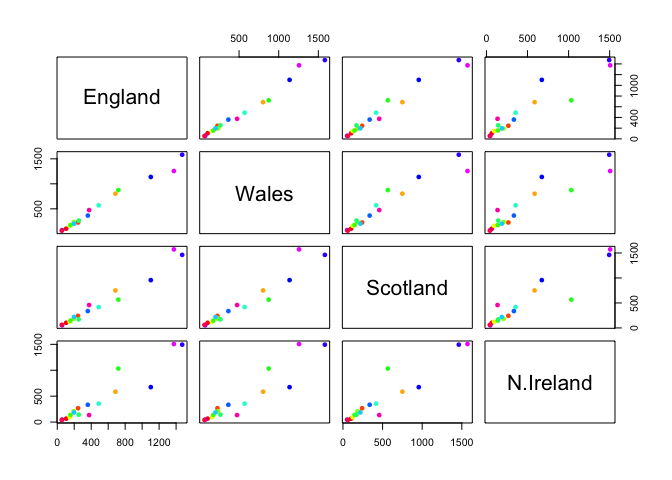
Main point: It can be difficult to spot major trends and patterns even in relatively small multivariate datasets (here we only have 17 dimensions, typically we have 1000s).
PCA to the rescue
The main function in “base” R for PCA is called prcomp()
I will take the transpose of our data so the “food” are in the columns:
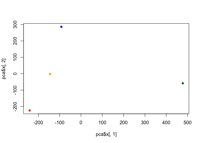
pca <- prcomp(t(x))
summary(pca)
Importance of components:
                            PC1      PC2      PC3       PC4
Standard deviation     324.1502 212.7478 73.87622 2.921e-14
Proportion of Variance   0.6744   0.2905  0.03503 0.000e+00
Cumulative Proportion    0.6744   0.9650  1.00000 1.000e+00
cols <- c("orange", "red", "blue", "darkgreen")
plot(pca$x[,1], pca$x[,2], col=cols, pch=16)
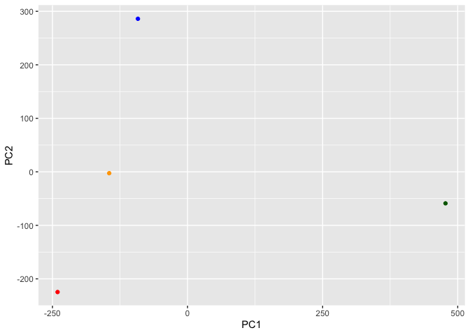
library(ggplot2)
ggplot(pca$x) +
  aes(PC1, PC2) +
  geom_point(col=cols)
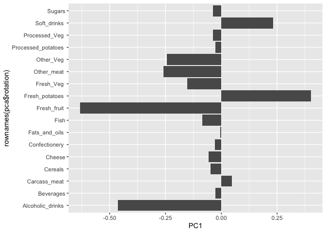
ggplot(pca$rotation) +
  aes(PC1, rownames(pca$rotation)) +
  geom_col()
PCA looks super useful and we will come back to describe this further next day ;-)