Blinda's Class
Classwork for BIMM143
Lab 08 Breast Cancer Analysis Mini Project
Blinda Sui (PID: A17117043)
- Background
- Data import
- Data Exploration
- Principal Component Analysis (PCA)
- PCA Scree-plot
- hierarchical clustering
- Combining methods (PCA and CLustering)
- 5. Combining Methods
- 6. Sensitivity/Specificity
- 7. Prediction
Background
The goal of this mini-project is for you to explore a complete analysis using the unsupervised learning techniques covered in class. You’ll extend what you’ve learned by combining PCA as a preprocessing step to clustering using data that consist of measurements of cell nuclei of human breast masses. This expands on our RNA-Seq analysis from last day.
The data itself comes from the Wisconsin Breast Cancer Diagnostic Data Set first reported by K. P. Benne and O. L. Mangasarian: “Robust Linear Programming Discrimination of Two Linearly Inseparable Sets”.
Values in this data set describe characteristics of the cell nuclei present in digitized images of a fine needle aspiration (FNA) of a breast mass.
Data import
Data was downloaded from the class website as a CSV file.
wisc.df <- read.csv("WisconsinCancer.csv", row.names=1)
head(wisc.df)
         diagnosis radius_mean texture_mean perimeter_mean area_mean
842302           M       17.99        10.38         122.80    1001.0
842517           M       20.57        17.77         132.90    1326.0
84300903         M       19.69        21.25         130.00    1203.0
84348301         M       11.42        20.38          77.58     386.1
84358402         M       20.29        14.34         135.10    1297.0
843786           M       12.45        15.70          82.57     477.1
         smoothness_mean compactness_mean concavity_mean concave.points_mean
842302           0.11840          0.27760         0.3001             0.14710
842517           0.08474          0.07864         0.0869             0.07017
84300903         0.10960          0.15990         0.1974             0.12790
84348301         0.14250          0.28390         0.2414             0.10520
84358402         0.10030          0.13280         0.1980             0.10430
843786           0.12780          0.17000         0.1578             0.08089
         symmetry_mean fractal_dimension_mean radius_se texture_se perimeter_se
842302          0.2419                0.07871    1.0950     0.9053        8.589
842517          0.1812                0.05667    0.5435     0.7339        3.398
84300903        0.2069                0.05999    0.7456     0.7869        4.585
84348301        0.2597                0.09744    0.4956     1.1560        3.445
84358402        0.1809                0.05883    0.7572     0.7813        5.438
843786          0.2087                0.07613    0.3345     0.8902        2.217
         area_se smoothness_se compactness_se concavity_se concave.points_se
842302    153.40      0.006399        0.04904      0.05373           0.01587
842517     74.08      0.005225        0.01308      0.01860           0.01340
84300903   94.03      0.006150        0.04006      0.03832           0.02058
84348301   27.23      0.009110        0.07458      0.05661           0.01867
84358402   94.44      0.011490        0.02461      0.05688           0.01885
843786     27.19      0.007510        0.03345      0.03672           0.01137
         symmetry_se fractal_dimension_se radius_worst texture_worst
842302       0.03003             0.006193        25.38         17.33
842517       0.01389             0.003532        24.99         23.41
84300903     0.02250             0.004571        23.57         25.53
84348301     0.05963             0.009208        14.91         26.50
84358402     0.01756             0.005115        22.54         16.67
843786       0.02165             0.005082        15.47         23.75
         perimeter_worst area_worst smoothness_worst compactness_worst
842302            184.60     2019.0           0.1622            0.6656
842517            158.80     1956.0           0.1238            0.1866
84300903          152.50     1709.0           0.1444            0.4245
84348301           98.87      567.7           0.2098            0.8663
84358402          152.20     1575.0           0.1374            0.2050
843786            103.40      741.6           0.1791            0.5249
         concavity_worst concave.points_worst symmetry_worst
842302            0.7119               0.2654         0.4601
842517            0.2416               0.1860         0.2750
84300903          0.4504               0.2430         0.3613
84348301          0.6869               0.2575         0.6638
84358402          0.4000               0.1625         0.2364
843786            0.5355               0.1741         0.3985
         fractal_dimension_worst
842302                   0.11890
842517                   0.08902
84300903                 0.08758
84348301                 0.17300
84358402                 0.07678
843786                   0.12440
Data Exploration
The first column diagnosis is the expert opinion on the sample
(i.e. patient FNA).
head(wisc.df$diagnosis)
[1] "M" "M" "M" "M" "M" "M"
Remove the diagnosis from data for subsequent analysis
#remove the first (diagnosis) column
wisc.data <- wisc.df[,-1]
#[ ]: subsetting R objects, including data frames, vectors, and matrices.
#,: [rows, columns]
#-1: exclude the first column/row

dim(wisc.data)
[1] 569 30
#dim(): get the dimensions of the wisc.data object - returns a vector with two numbers: # of rows and # of columns
Store the diagnosis as a vector for use later when we compare our results to those from experts in the field.
diagnosis <- factor(wisc.df$diagnosis)
Q1.How many observations are in this dataset?
There are 569 observations/patients in the dataset
nrow(wisc.data)
[1] 569
Q2. How many of the observations have a malignant diagnosis?
table(wisc.df$diagnosis)
  B   M
357 212
#table(): output a table displaying the counts of each unique value present in the diagnosis column of your wisc.df data frame
Q3. How many variables/features in the data are suffixed with _mean?
colnames(wisc.data)
 [1] "radius_mean"             "texture_mean"
 [3] "perimeter_mean"          "area_mean"
 [5] "smoothness_mean"         "compactness_mean"
 [7] "concavity_mean"          "concave.points_mean"
 [9] "symmetry_mean"           "fractal_dimension_mean"
[11] "radius_se"               "texture_se"
[13] "perimeter_se"            "area_se"
[15] "smoothness_se"           "compactness_se"
[17] "concavity_se"            "concave.points_se"
[19] "symmetry_se"             "fractal_dimension_se"
[21] "radius_worst"            "texture_worst"
[23] "perimeter_worst"         "area_worst"
[25] "smoothness_worst"        "compactness_worst"
[27] "concavity_worst"         "concave.points_worst"
[29] "symmetry_worst"          "fractal_dimension_worst"
#colnames(): output a character vector containing the names of the columns.
#colnames(wisc.data)
length(grep("_mean", colnames(wisc.data)))
[1] 10
#grep(): searches for matches to a specified pattern within each element of a character vector x.
#length(): how many
Principal Component Analysis (PCA)
The prcomp() function to do PCA has a scale=FALSE default. In
general we nearly always want to set this to TRUE so our analysis is not
dominated by columns/variables in our dataset that have high standard
deviation and mean when compared to others just because the units of
measurement are on different scales/units.
scale: a logical value indicating whether the variables should be scaled to have unit variance before the analysis take place. center: a logical value (or a vector of values) that determines whether the variables in the dataset should have their mean subtracted, or “zero-centered,” before the principal component analysis (PCA) is performed.
wisc.pr <- prcomp(wisc.data, scale = TRUE)
summary(wisc.pr)
Importance of components:
                          PC1    PC2     PC3     PC4     PC5     PC6     PC7
Standard deviation     3.6444 2.3857 1.67867 1.40735 1.28403 1.09880 0.82172
Proportion of Variance 0.4427 0.1897 0.09393 0.06602 0.05496 0.04025 0.02251
Cumulative Proportion  0.4427 0.6324 0.72636 0.79239 0.84734 0.88759 0.91010
                           PC8    PC9    PC10   PC11    PC12    PC13    PC14
Standard deviation     0.69037 0.6457 0.59219 0.5421 0.51104 0.49128 0.39624
Proportion of Variance 0.01589 0.0139 0.01169 0.0098 0.00871 0.00805 0.00523
Cumulative Proportion  0.92598 0.9399 0.95157 0.9614 0.97007 0.97812 0.98335
                          PC15    PC16    PC17    PC18    PC19    PC20   PC21
Standard deviation     0.30681 0.28260 0.24372 0.22939 0.22244 0.17652 0.1731
Proportion of Variance 0.00314 0.00266 0.00198 0.00175 0.00165 0.00104 0.0010
Cumulative Proportion  0.98649 0.98915 0.99113 0.99288 0.99453 0.99557 0.9966
                          PC22    PC23   PC24    PC25    PC26    PC27    PC28
Standard deviation     0.16565 0.15602 0.1344 0.12442 0.09043 0.08307 0.03987
Proportion of Variance 0.00091 0.00081 0.0006 0.00052 0.00027 0.00023 0.00005
Cumulative Proportion  0.99749 0.99830 0.9989 0.99942 0.99969 0.99992 0.99997
                          PC29    PC30
Standard deviation     0.02736 0.01153
Proportion of Variance 0.00002 0.00000
Cumulative Proportion  1.00000 1.00000
Q4. From your results, what proportion of the original variance is captured by the first principal components (PC1)?
# variance proportions from the PCA object
prop_var <- (wisc.pr$sdev^2) / sum(wisc.pr$sdev^2)
cum_var  <- cumsum(prop_var)

# Q4: proportion captured by PC1
Q4_PC1 <- prop_var[1]
round(Q4_PC1, 4)
[1] 0.4427
Q5. How many principal components (PCs) are required to describe at least 70% of the original variance in the data?
# Q5: # of PCs for at least 70% variance
Q5_n70 <- which(cum_var >= 0.70)[1]
Q5_n70
[1] 3
Q6. How many principal components (PCs) are required to describe at least 90% of the original variance in the data?
# Q6: # of PCs for at least 90% variance
Q6_n90 <- which(cum_var >= 0.90)[1]
Q6_n90
[1] 7
PCA Score Plot
Q7. What stands out to you about this plot? Is it easy or difficult to understand? Why?
# Basic biplot of the PCA you already computed
biplot(wisc.pr, scale = 0, cex = 0.5, col = c("grey50","tomato"),
       xlab = "PC1", ylab = "PC2",
       main = "Biplot: Wisconsin Cancer PCA (PC1 vs PC2)")
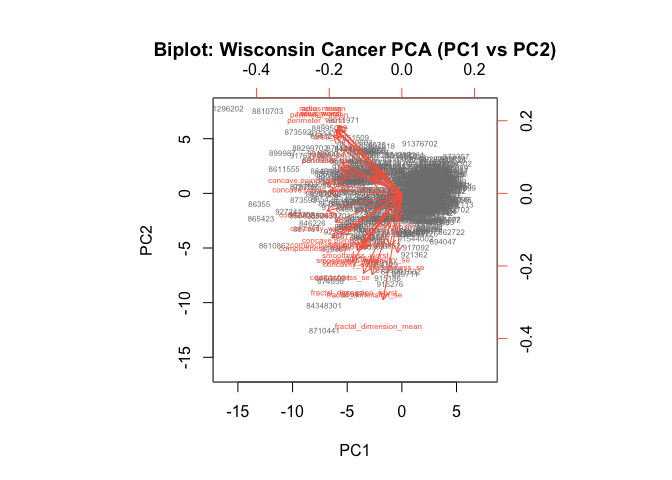
- What stands out:
- Hundreds of patient points stacked on top of each other near the center and stretched along PC1.
- A dense “starburst” of red arrows (one for each feature) pointing roughly in similar directions for highly correlated features (e.g., many radius/area/perimeter/texture variants).
- PC1 explains a big chunk of the variance, so separation is mostly left–right along PC1.
- It’s difficult to understand:
- Overplotting: ~500+ observations + ~30 variables means points and labels overlap; you can’t tell individuals apart.
- Label clutter: Variable names printed on top of arrows become unreadable.
- Mixed encodings: Scores and loadings share the same panel and axes, which asks you to interpret two different things at once (sample positions and variable directions).
- Arbitrary sign: The direction of PCs (and thus arrow orientations) can flip without changing meaning, which can be confusing when comparing plots.
- No class info: Diagnosis (M/B) isn’t shown by default, so you can’t judge class separation from this plot alone.
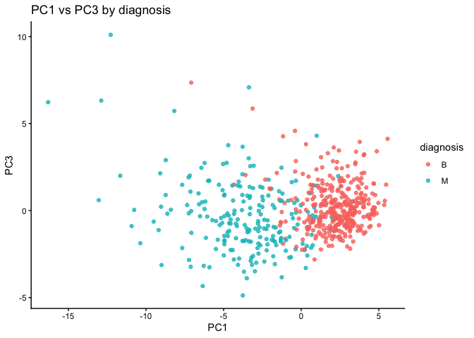
Q8. Generate a similar plot for principal components 1 and 3. What do you notice about these plots?
# Make a data frame of PC scores and add the labels
df <- as.data.frame(wisc.pr$x)
df$diagnosis <- diagnosis   # factor

# PC1 vs PC3
library(ggplot2)
ggplot(df, aes(PC1, PC3, color = diagnosis)) +
  geom_point(alpha = 0.8) +
  labs(title = "PC1 vs PC3 by diagnosis",
       x = "PC1", y = "PC3") +
  theme_classic()
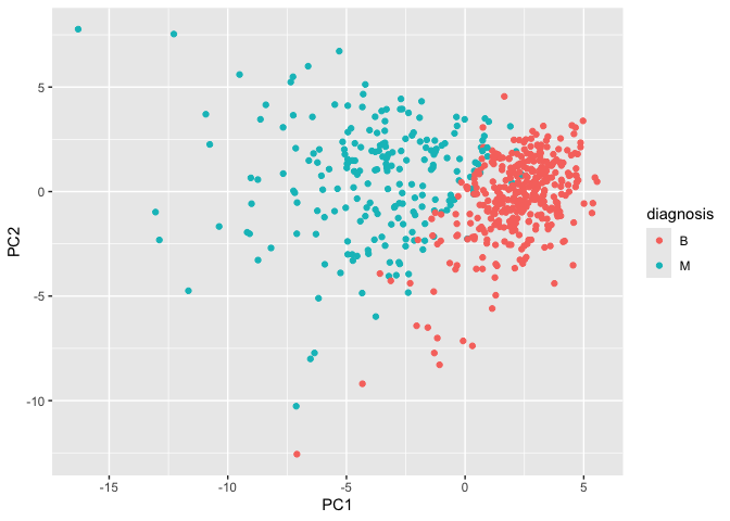
The main PC result figure is called a “score plot” or “PC plot” or “ordination plot”…
library(ggplot2)

ggplot(wisc.pr$x) +
  aes(PC1, PC2, col = diagnosis) +
  geom_point()
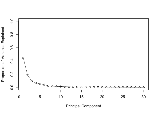
PCA Scree-plot
A plot of how much variance each PC captures
pr.var <- wisc.pr$sdev^2
head(pr.var)
[1] 13.281608 5.691355 2.817949 1.980640 1.648731 1.207357
# Variance explained by each principal component: pve
pve <- pr.var / sum(pr.var)

# Plot variance explained for each principal component
plot(pve, xlab = "Principal Component",
     ylab = "Proportion of Variance Explained",
     ylim = c(0, 1), type = "o")
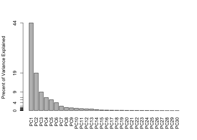
# Alternative scree plot of the same data, note data driven y-axis
barplot(pve, ylab = "Precent of Variance Explained",
     names.arg=paste0("PC",1:length(pve)), las=2, axes = FALSE)
axis(2, at=pve, labels=round(pve,2)*100 )
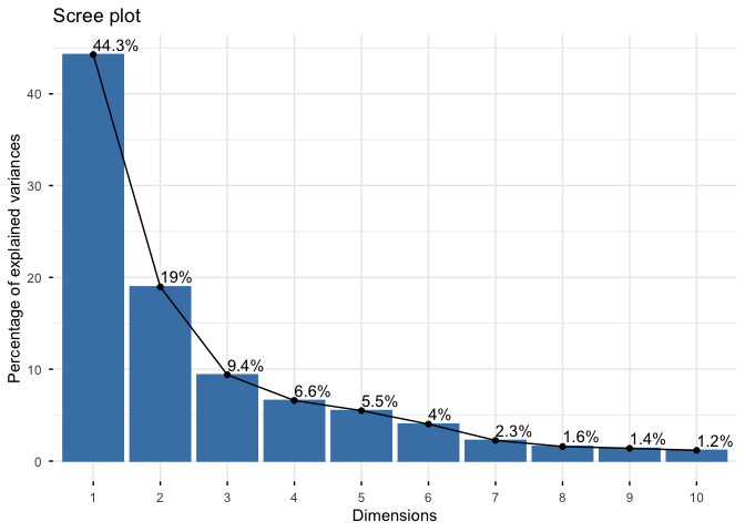
## ggplot based graph
#install.packages("factoextra")
library(factoextra)
Welcome! Want to learn more? See two factoextra-related books at https://goo.gl/ve3WBa
fviz_eig(wisc.pr, addlabels = TRUE)
Warning in geom_bar(stat = "identity", fill = barfill, color = barcolor, :
Ignoring empty aesthetic: `width`.
Communicating PCA results
Q9. For the first principal component, what is the component of the loading vector (i.e. wisc.pr$rotation[,1]) for the feature concave.points_mean?
wisc.pr$rotation["concave.points_mean", "PC1"]
[1] -0.2608538
Q10. What is the minimum number of principal components required to explain 80% of the variance of the data?
summary(wisc.pr)
Importance of components:
                          PC1    PC2     PC3     PC4     PC5     PC6     PC7
Standard deviation     3.6444 2.3857 1.67867 1.40735 1.28403 1.09880 0.82172
Proportion of Variance 0.4427 0.1897 0.09393 0.06602 0.05496 0.04025 0.02251
Cumulative Proportion  0.4427 0.6324 0.72636 0.79239 0.84734 0.88759 0.91010
                           PC8    PC9    PC10   PC11    PC12    PC13    PC14
Standard deviation     0.69037 0.6457 0.59219 0.5421 0.51104 0.49128 0.39624
Proportion of Variance 0.01589 0.0139 0.01169 0.0098 0.00871 0.00805 0.00523
Cumulative Proportion  0.92598 0.9399 0.95157 0.9614 0.97007 0.97812 0.98335
                          PC15    PC16    PC17    PC18    PC19    PC20   PC21
Standard deviation     0.30681 0.28260 0.24372 0.22939 0.22244 0.17652 0.1731
Proportion of Variance 0.00314 0.00266 0.00198 0.00175 0.00165 0.00104 0.0010
Cumulative Proportion  0.98649 0.98915 0.99113 0.99288 0.99453 0.99557 0.9966
                          PC22    PC23   PC24    PC25    PC26    PC27    PC28
Standard deviation     0.16565 0.15602 0.1344 0.12442 0.09043 0.08307 0.03987
Proportion of Variance 0.00091 0.00081 0.0006 0.00052 0.00027 0.00023 0.00005
Cumulative Proportion  0.99749 0.99830 0.9989 0.99942 0.99969 0.99992 0.99997
                          PC29    PC30
Standard deviation     0.02736 0.01153
Proportion of Variance 0.00002 0.00000
Cumulative Proportion  1.00000 1.00000
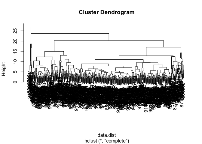
hierarchical clustering
Just clustering the original data is not very informative or helpful.
data.scaled <- scale(wisc.data)
data.dist <- dist(data.scaled)
wisc.hclust <- hclust(data.dist)
View the clustering dendrogram result
plot(wisc.hclust)
wisc.hclust.clusters <- cutree(wisc.hclust, k=4)
table(wisc.hclust.clusters)
wisc.hclust.clusters
  1   2   3   4
177   7 383   2
table(wisc.hclust.clusters, diagnosis)
                    diagnosis
wisc.hclust.clusters   B   M
                   1  12 165
                   2   2   5
                   3 343  40
                   4   0   2
Combining methods (PCA and CLustering)
Clustering the origional data was not very productive. THe PCA results looked promising. Here we combine these methods by clustering from our PCA results. In other words “clustering in PC space”… > Q11. Using the plot() and abline() functions, what is the height at which the clustering model has 4 clusters?
## Take the first 3 PCs
dist.pc <- dist(wisc.pr$x[, 1:3])
wisc.pr.hclust <- hclust(dist.pc, method = "ward.D2")
View the tree…
plot(wisc.pr.hclust)
abline(h = 70, col="red")

To get our clustering membership vector (i.e. our main clustering result) we “cut” the tree at a desired height or to yield a desired number of “k groups.
grps <- cutree(wisc.pr.hclust, h = 70)
table(grps)
grps
  1   2
203 366
How does this clustering grps compare to the expert diagnosis
table(grps, diagnosis)
    diagnosis
grps   B   M
   1  24 179
   2 333  33
Q12. Can you find a better cluster vs diagnoses match by cutting into a different number of clusters between 2 and 10?
# helper: map clusters -> labels by majority vote, then accuracy/sens/spec
cluster_metrics <- function(cl, truth = diagnosis) {
  tab <- table(cl, truth)
  map <- apply(tab, 1, function(r) names(which.max(r)))
  pred <- factor(map[as.character(cl)], levels = levels(truth))
  cm <- table(pred, truth)
  acc <- mean(pred == truth)
  sens <- cm["M","M"] / sum(cm[ , "M"])        # TPR for Malignant
  spec <- cm["B","B"] / sum(cm[ , "B"])        # TNR for Benign
  list(acc = acc, sens = sens, spec = spec, cm = cm)
}

# evaluate cutting the PC-space tree at k = 2:10
ks <- 2:10
pc_k_results <- lapply(ks, function(k){
  cl <- cutree(wisc.pr.hclust, k = k)
  cluster_metrics(cl)
})
acc_by_k <- sapply(pc_k_results, `[[`, "acc")
data.frame(k = ks, accuracy = round(acc_by_k, 4))
   k accuracy
1  2   0.8998
2  3   0.8998
3  4   0.8998
4  5   0.8998
5  6   0.9139
6  7   0.9139
7  8   0.9139
8  9   0.9139
9 10   0.9139
Q13. Which method gives your favorite results for the same data.dist dataset? Explain your reasoning.
methods <- c("single", "complete", "average", "ward.D2")
link_res <- lapply(methods, function(m) {
  hc <- hclust(data.dist, method = m)
  cluster_metrics(cutree(hc, k = 2))   # two true classes
})
data.frame(
  method = methods,
  accuracy = sapply(link_res, `[[`, "acc"),
  sensitivity = sapply(link_res, `[[`, "sens"),
  specificity = sapply(link_res, `[[`, "spec")
)
    method  accuracy sensitivity specificity
1   single 0.6309315 0.009433962   1.0000000
2 complete 0.6309315 0.009433962   1.0000000
3  average 0.6326889 0.014150943   1.0000000
4  ward.D2 0.8804921 0.773584906   0.9439776
K-means clustering
Q14. How well does k-means separate the two diagnoses? How does it compare to your hclust results?
set.seed(1)
wisc.km <- kmeans(data.scaled, centers = 2, nstart = 50)

km_res  <- cluster_metrics(wisc.km$cluster)
hc2_res <- cluster_metrics(cutree(wisc.hclust, k = 2))

km_res$cm; round(c(km_acc = km_res$acc, km_sens = km_res$sens, km_spec = km_res$spec), 3)
    truth
pred   B   M
   B 343  37
   M  14 175

 km_acc km_sens km_spec
  0.910   0.825   0.961
hc2_res$cm; round(c(hc_acc = hc2_res$acc, hc_sens = hc2_res$sens, hc_spec = hc2_res$spec), 3)
    truth
pred   B   M
   B 357 210
   M   0   2

 hc_acc hc_sens hc_spec
  0.631   0.009   1.000
- k-means reaches accuracy ___ (sens **, spec **), compared with hierarchical (k=2) accuracy ___ (sens **, spec **). Thus, k-means [wins/loses/is comparable].
5. Combining Methods
Q15. How well does the newly created model with four clusters separate out the two diagnoses?
hc4_res <- cluster_metrics(wisc.hclust.clusters)
hc4_res$cm
    truth
pred   B   M
   B 343  40
   M  14 172
round(c(acc = hc4_res$acc, sens = hc4_res$sens, spec = hc4_res$spec), 3)
  acc  sens  spec
0.905 0.811 0.961
- With k=4, accuracy ___ (sens **, spec **). Two of the four clusters are mostly ___; the split adds little label purity over k=2
Q16. How well do the k-means and hierarchical clustering models you created in previous sections (i.e. before PCA) do in terms of separating the diagnoses? Again, use the table() function to compare the output of each model (wisc.km$cluster and wisc.hclust.clusters) with the vector containing the actual diagnoses.
# Plain cross-tabs (what the question asks for)
table(wisc.km$cluster, diagnosis)
   diagnosis
      B   M
  1 343  37
  2  14 175
table(wisc.hclust.clusters, diagnosis)
                    diagnosis
wisc.hclust.clusters   B   M
                   1  12 165
                   2   2   5
                   3 343  40
                   4   0   2
6. Sensitivity/Specificity
Sensitivity: TP/(TP+FN) Specificity: TN/(TN+FN)
Q17. Which of your analysis procedures resulted in a clustering model with the best specificity? How about sensitivity?
# Collect all contenders you tried
summary_df <- rbind(
  cbind(model = "hclust complete k=2",  t(unlist(hc2_res[c("acc","sens","spec")]))),
  cbind(model = "hclust complete k=4",  t(unlist(hc4_res[c("acc","sens","spec")]))),
  cbind(model = "kmeans k=2",          t(unlist(km_res[c("acc","sens","spec")]))),
  cbind(model = sprintf("PC Ward.D2 k=%d", ks[which.max(acc_by_k)]),
        t(unlist(pc_k_results[[which.max(acc_by_k)]][c("acc","sens","spec")])))
)
summary_df
     model                 acc                 sens
[1,] "hclust complete k=2" "0.630931458699473" "0.00943396226415094"
[2,] "hclust complete k=4" "0.905096660808436" "0.811320754716981"
[3,] "kmeans k=2"          "0.9103690685413"   "0.825471698113208"
[4,] "PC Ward.D2 k=6"      "0.913884007029877" "0.820754716981132"
     spec
[1,] "1"
[2,] "0.96078431372549"
[3,] "0.96078431372549"
[4,] "0.969187675070028"
- Best specificity (fewest benign→malignant false positives) came from ___ (spec = **); best sensitivity (fewest malignant misses) came from ** (sens = **). I’d choose ** depending on whether I want to minimize false alarms or missed cancers.
7. Prediction
We can use our PCA model for prediction with new input patient samples.
#url <- "new_samples.csv"
url <- "https://tinyurl.com/new-samples-CSV"
new <- read.csv(url)
npc <- predict(wisc.pr, newdata=new)
npc
           PC1       PC2        PC3        PC4       PC5        PC6        PC7
[1,]  2.576616 -3.135913  1.3990492 -0.7631950  2.781648 -0.8150185 -0.3959098
[2,] -4.754928 -3.009033 -0.1660946 -0.6052952 -1.140698 -1.2189945  0.8193031
            PC8       PC9       PC10      PC11      PC12      PC13     PC14
[1,] -0.2307350 0.1029569 -0.9272861 0.3411457  0.375921 0.1610764 1.187882
[2,] -0.3307423 0.5281896 -0.4855301 0.7173233 -1.185917 0.5893856 0.303029
          PC15       PC16        PC17        PC18        PC19       PC20
[1,] 0.3216974 -0.1743616 -0.07875393 -0.11207028 -0.08802955 -0.2495216
[2,] 0.1299153  0.1448061 -0.40509706  0.06565549  0.25591230 -0.4289500
           PC21       PC22       PC23       PC24        PC25         PC26
[1,]  0.1228233 0.09358453 0.08347651  0.1223396  0.02124121  0.078884581
[2,] -0.1224776 0.01732146 0.06316631 -0.2338618 -0.20755948 -0.009833238
             PC27        PC28         PC29         PC30
[1,]  0.220199544 -0.02946023 -0.015620933  0.005269029
[2,] -0.001134152  0.09638361  0.002795349 -0.019015820
plot(wisc.pr$x[,1:2], col=diagnosis)
points(npc[,1], npc[,2], col="blue", pch=16, cex=3)
text(npc[,1], npc[,2], c(1,2), col="white")
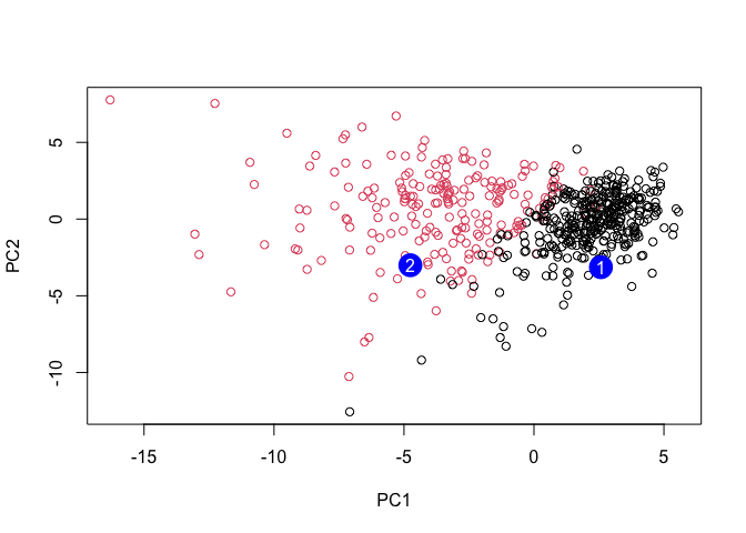
Q18. Which of these new patients should we prioritize for follow up based on your results?
Patient 1 falls on the malignant side of PC1 and is closest to the malignant centroid in PC space; prioritize Patient 1 for follow-up.