Blinda's Class
Classwork for BIMM143
Lab 10: Halloween mini project
Blinda Sui (PID: A17117043)
- Data Import
- Quick overview of the dataset
- Overall Candy Rankings
- Winpercent and Pricepercent
- Exploring the corelation structure
- Principal Component Analysis
As it is nearly Halloween and th ehalf way point in the quarter, let’s do a mini project at help us figure out the best candy!
Our come from the 538 website and is available as a CSV file:
Data Import
candy <- read.csv("candy-data.csv", row.names = 1)
head(candy)
             chocolate fruity caramel peanutyalmondy nougat crispedricewafer
100 Grand            1      0       1              0      0                1
3 Musketeers         1      0       0              0      1                0
One dime             0      0       0              0      0                0
One quarter          0      0       0              0      0                0
Air Heads            0      1       0              0      0                0
Almond Joy           1      0       0              1      0                0
             hard bar pluribus sugarpercent pricepercent winpercent
100 Grand       0   1        0        0.732        0.860   66.97173
3 Musketeers    0   1        0        0.604        0.511   67.60294
One dime        0   0        0        0.011        0.116   32.26109
One quarter     0   0        0        0.011        0.511   46.11650
Air Heads       0   0        0        0.906        0.511   52.34146
Almond Joy      0   1        0        0.465        0.767   50.34755
flextable::flextable(head(candy, 10))

Q1. How many different candy types are in this dataset?
nrow(candy)
[1] 85
candy |>
  nrow()
[1] 85
library(tidyverse)
── Attaching core tidyverse packages ──────────────────────── tidyverse 2.0.0 ──
✔ dplyr     1.1.4     ✔ readr     2.1.5
✔ forcats   1.0.1     ✔ stringr   1.5.2
✔ ggplot2   4.0.0     ✔ tibble    3.3.0
✔ lubridate 1.9.4     ✔ tidyr     1.3.1
✔ purrr     1.1.0
── Conflicts ────────────────────────────────────────── tidyverse_conflicts() ──
✖ dplyr::filter() masks stats::filter()
✖ dplyr::lag()    masks stats::lag()
ℹ Use the conflicted package (<http://conflicted.r-lib.org/>) to force all conflicts to become errors
candy %>%
  nrow()
[1] 85
Q2. How many fruity candy types are in the dataset?
sum(candy$fruity)
[1] 38
Q3. What is your favorite candy in the dataset and what is it’s winpercent value?
My favorite winpercent
candy["Twix", ]$winpercent
[1] 81.64291
library(dplyr)

candy |>
  filter(rownames(candy) == "Boston Baked Beans") |>
  select(winpercent)
                   winpercent
Boston Baked Beans   23.41782
Q4. What is the winpercent value for “Kit Kat”?
candy["Kit Kat", ]$winpercent
[1] 76.7686
Q5. What is the winpercent value for “Tootsie Roll Snack Bars”?
candy["Tootsie Roll Snack Bars", ]$winpercent
[1] 49.6535
Quick overview of the dataset
#It is a modern, tidyverse-friendly alternative to the base R function summary()
skimr::skim(candy)
| Name | candy |
| Number of rows | 85 |
| Number of columns | 12 |
| _______________________ | |
| Column type frequency: | |
| numeric | 12 |
| ________________________ | |
| Group variables | None |
Data summary
Variable type: numeric
| skim_variable | n_missing | complete_rate | mean | sd | p0 | p25 | p50 | p75 | p100 | hist |
|---|---|---|---|---|---|---|---|---|---|---|
| chocolate | 0 | 1 | 0.44 | 0.50 | 0.00 | 0.00 | 0.00 | 1.00 | 1.00 | ▇▁▁▁▆ |
| fruity | 0 | 1 | 0.45 | 0.50 | 0.00 | 0.00 | 0.00 | 1.00 | 1.00 | ▇▁▁▁▆ |
| caramel | 0 | 1 | 0.16 | 0.37 | 0.00 | 0.00 | 0.00 | 0.00 | 1.00 | ▇▁▁▁▂ |
| peanutyalmondy | 0 | 1 | 0.16 | 0.37 | 0.00 | 0.00 | 0.00 | 0.00 | 1.00 | ▇▁▁▁▂ |
| nougat | 0 | 1 | 0.08 | 0.28 | 0.00 | 0.00 | 0.00 | 0.00 | 1.00 | ▇▁▁▁▁ |
| crispedricewafer | 0 | 1 | 0.08 | 0.28 | 0.00 | 0.00 | 0.00 | 0.00 | 1.00 | ▇▁▁▁▁ |
| hard | 0 | 1 | 0.18 | 0.38 | 0.00 | 0.00 | 0.00 | 0.00 | 1.00 | ▇▁▁▁▂ |
| bar | 0 | 1 | 0.25 | 0.43 | 0.00 | 0.00 | 0.00 | 0.00 | 1.00 | ▇▁▁▁▂ |
| pluribus | 0 | 1 | 0.52 | 0.50 | 0.00 | 0.00 | 1.00 | 1.00 | 1.00 | ▇▁▁▁▇ |
| sugarpercent | 0 | 1 | 0.48 | 0.28 | 0.01 | 0.22 | 0.47 | 0.73 | 0.99 | ▇▇▇▇▆ |
| pricepercent | 0 | 1 | 0.47 | 0.29 | 0.01 | 0.26 | 0.47 | 0.65 | 0.98 | ▇▇▇▇▆ |
| winpercent | 0 | 1 | 50.32 | 14.71 | 22.45 | 39.14 | 47.83 | 59.86 | 84.18 | ▃▇▆▅▂ |
Q6. Is there any variable/column that looks to be on a different scale to the majority of the other columns in the dataset?
The winpercent is on a 0-100 scale the rest are 0-1 scale
Q7. What do you think a zero and one represent for the candy$chocolate column?
That the candy does not contain chocolate
Q8. Plot a histogram of winpercent values
library(ggplot2)

ggplot(candy) +
  aes(winpercent) +
  geom_histogram(bins=20)
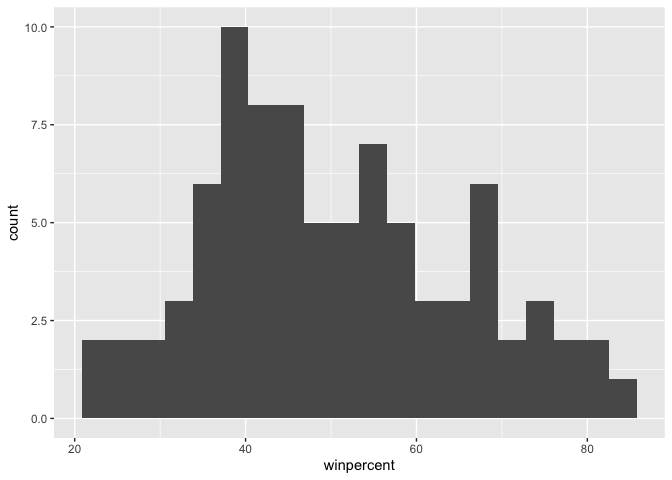
Q9. Is the distribution of winpercent values symmetrical?
ggplot(candy) +
  aes(winpercent) +
  geom_density()
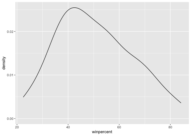
Q10. Is the center of the distribution above or below 50%?
mean(candy$winpercent)
[1] 50.31676
summary(candy$winpercent)
   Min. 1st Qu.  Median    Mean 3rd Qu.    Max.
  22.45   39.14   47.83   50.32   59.86   84.18
Q11. On average is chocolate candy higher or lower ranked than fruit candy?
# 1. Find all chocolate candy in the dataset
# 2. Find their winpercent values
# 3. Calculate the mean of these values

# 4-6. DO the same for fruity candy
# 7. compare mean winpercents of chocolate vs fruity
# 8. Pick the highest as the winnder

choc.inds <- candy$chocolate == 1
choc.win <- candy[choc.inds, ]$winpercent
choc.mean <- mean(choc.win)
choc.mean
[1] 60.92153
mean(candy[candy$chocolate==1,]$winpercent)
[1] 60.92153
mean(candy[candy$fruity==1,]$winpercent)
[1] 44.11974
fruit.ind <- candy$fruity==1
fruit.win <- candy[fruit.ind,]$winpercent
fruit.mean <- mean(fruit.win)
fruit.mean
[1] 44.11974
candy |>
  filter(chocolate==1) |>
  select(winpercent)
                            winpercent
100 Grand                     66.97173
3 Musketeers                  67.60294
Almond Joy                    50.34755
Baby Ruth                     56.91455
Charleston Chew               38.97504
Hershey's Kisses              55.37545
Hershey's Krackel             62.28448
Hershey's Milk Chocolate      56.49050
Hershey's Special Dark        59.23612
Junior Mints                  57.21925
Kit Kat                       76.76860
Peanut butter M&M's           71.46505
M&M's                         66.57458
Milk Duds                     55.06407
Milky Way                     73.09956
Milky Way Midnight            60.80070
Milky Way Simply Caramel      64.35334
Mounds                        47.82975
Mr Good Bar                   54.52645
Nestle Butterfinger           70.73564
Nestle Crunch                 66.47068
Peanut M&Ms                   69.48379
Reese's Miniatures            81.86626
Reese's Peanut Butter cup     84.18029
Reese's pieces                73.43499
Reese's stuffed with pieces   72.88790
Rolo                          65.71629
Sixlets                       34.72200
Nestle Smarties               37.88719
Snickers                      76.67378
Snickers Crisper              59.52925
Tootsie Pop                   48.98265
Tootsie Roll Juniors          43.06890
Tootsie Roll Midgies          45.73675
Tootsie Roll Snack Bars       49.65350
Twix                          81.64291
Whoppers                      49.52411
Q12. Is this difference statistically significant?
t.test(choc.win, fruit.win)
    Welch Two Sample t-test

data:  choc.win and fruit.win
t = 6.2582, df = 68.882, p-value = 2.871e-08
alternative hypothesis: true difference in means is not equal to 0
95 percent confidence interval:
 11.44563 22.15795
sample estimates:
mean of x mean of y
 60.92153  44.11974
Overall Candy Rankings
Q13. What are the five least liked candy types in this set?
candy |>
  arrange(winpercent) |>
  head(5)
                   chocolate fruity caramel peanutyalmondy nougat
Nik L Nip                  0      1       0              0      0
Boston Baked Beans         0      0       0              1      0
Chiclets                   0      1       0              0      0
Super Bubble               0      1       0              0      0
Jawbusters                 0      1       0              0      0
                   crispedricewafer hard bar pluribus sugarpercent pricepercent
Nik L Nip                         0    0   0        1        0.197        0.976
Boston Baked Beans                0    0   0        1        0.313        0.511
Chiclets                          0    0   0        1        0.046        0.325
Super Bubble                      0    0   0        0        0.162        0.116
Jawbusters                        0    1   0        1        0.093        0.511
                   winpercent
Nik L Nip            22.44534
Boston Baked Beans   23.41782
Chiclets             24.52499
Super Bubble         27.30386
Jawbusters           28.12744
ord.ind <- order(candy$winpercent)
head(candy[ord.ind,], 5)
                   chocolate fruity caramel peanutyalmondy nougat
Nik L Nip                  0      1       0              0      0
Boston Baked Beans         0      0       0              1      0
Chiclets                   0      1       0              0      0
Super Bubble               0      1       0              0      0
Jawbusters                 0      1       0              0      0
                   crispedricewafer hard bar pluribus sugarpercent pricepercent
Nik L Nip                         0    0   0        1        0.197        0.976
Boston Baked Beans                0    0   0        1        0.313        0.511
Chiclets                          0    0   0        1        0.046        0.325
Super Bubble                      0    0   0        0        0.162        0.116
Jawbusters                        0    1   0        1        0.093        0.511
                   winpercent
Nik L Nip            22.44534
Boston Baked Beans   23.41782
Chiclets             24.52499
Super Bubble         27.30386
Jawbusters           28.12744
Q14. What are the top 5 all time favorite candy types out of this set?
default = lowest to highest
candy |>
  arrange(winpercent) |>
  tail(5)
                          chocolate fruity caramel peanutyalmondy nougat
Snickers                          1      0       1              1      1
Kit Kat                           1      0       0              0      0
Twix                              1      0       1              0      0
Reese's Miniatures                1      0       0              1      0
Reese's Peanut Butter cup         1      0       0              1      0
                          crispedricewafer hard bar pluribus sugarpercent
Snickers                                 0    0   1        0        0.546
Kit Kat                                  1    0   1        0        0.313
Twix                                     1    0   1        0        0.546
Reese's Miniatures                       0    0   0        0        0.034
Reese's Peanut Butter cup                0    0   0        0        0.720
                          pricepercent winpercent
Snickers                         0.651   76.67378
Kit Kat                          0.511   76.76860
Twix                             0.906   81.64291
Reese's Miniatures               0.279   81.86626
Reese's Peanut Butter cup        0.651   84.18029
Q15. Make a first barplot of candy ranking based on winpercent values.
ggplot(candy) +
  aes(winpercent, rownames(candy)) +
  geom_col()
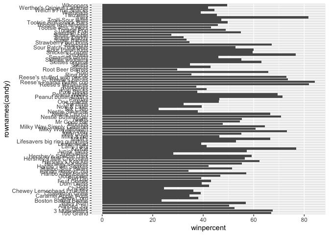
Q16. This is quite ugly, use the reorder() function to get the bars sorted by winpercent?
Add some color based on the “type of candy”
my_cols <- rep("black", nrow(candy)) #repeat number of candies I have
my_cols[as.logical(candy$chocolate)] <- "chocolate"
my_cols[as.logical(candy$fruity)] <- "red"
my_cols[as.logical(candy$bar)] <- "pink"
my_cols
 [1] "pink"      "pink"      "black"     "black"     "red"       "pink"
 [7] "pink"      "black"     "black"     "red"       "pink"      "red"
[13] "red"       "red"       "red"       "red"       "red"       "red"
[19] "red"       "black"     "red"       "red"       "chocolate" "pink"
[25] "pink"      "pink"      "red"       "chocolate" "pink"      "red"
[31] "red"       "red"       "chocolate" "chocolate" "red"       "chocolate"
[37] "pink"      "pink"      "pink"      "pink"      "pink"      "red"
[43] "pink"      "pink"      "red"       "red"       "pink"      "chocolate"
[49] "black"     "red"       "red"       "chocolate" "chocolate" "chocolate"
[55] "chocolate" "red"       "chocolate" "black"     "red"       "chocolate"
[61] "red"       "red"       "chocolate" "red"       "pink"      "pink"
[67] "red"       "red"       "red"       "red"       "black"     "black"
[73] "red"       "red"       "red"       "chocolate" "chocolate" "pink"
[79] "red"       "pink"      "red"       "red"       "red"       "black"
[85] "chocolate"
ggplot(candy) +
  aes(x = winpercent,
      y = reorder(rownames(candy), winpercent)) +
  geom_col(fill=my_cols)
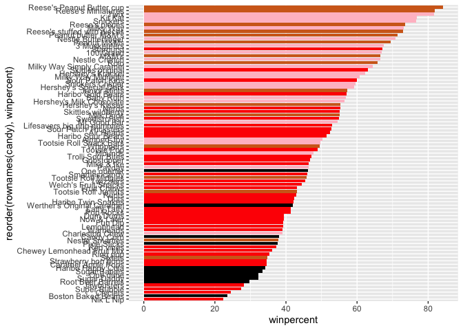
Q17. What is the worst ranked chocolate candy?
Sixlets
Q18. What is the best ranked fruity candy?
Starburst
Winpercent and Pricepercent
A plot with both variables/columns winpercent and pricepercent
library(ggrepel)

ggplot(candy) +
  aes(x = winpercent,
       y = pricepercent,
      label = rownames(candy)) +
  geom_point(col=my_cols) +
  geom_text_repel(max.overlaps = 7)
Warning: ggrepel: 45 unlabeled data points (too many overlaps). Consider
increasing max.overlaps
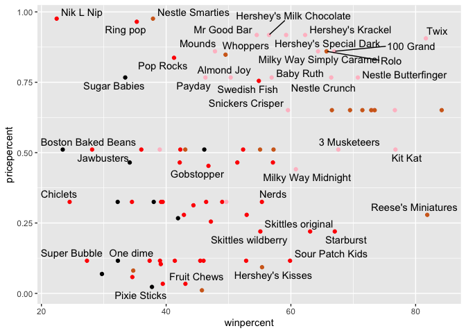
Q19. Which candy type is the highest ranked in terms of winpercent for the least money - i.e. offers the most bang for your buck?
Chocolate candy type
Q20. What are the top 5 most expensive candy types in the dataset and of these which is the least popular?
ord <- order(candy$pricepercent, decreasing = TRUE)
head( candy[ord,c(11,12)], n=5 )
                         pricepercent winpercent
Nik L Nip                       0.976   22.44534
Nestle Smarties                 0.976   37.88719
Ring pop                        0.965   35.29076
Hershey's Krackel               0.918   62.28448
Hershey's Milk Chocolate        0.918   56.49050
Exploring the corelation structure
Now that we’ve explored the dataset a little, we’ll see how the variables interact with one another. We’ll use correlation and view the results with the corrplot package to plot a correlation matrix.
library(corrplot)
corrplot 0.95 loaded
cij <- cor(candy)
corrplot(cij)
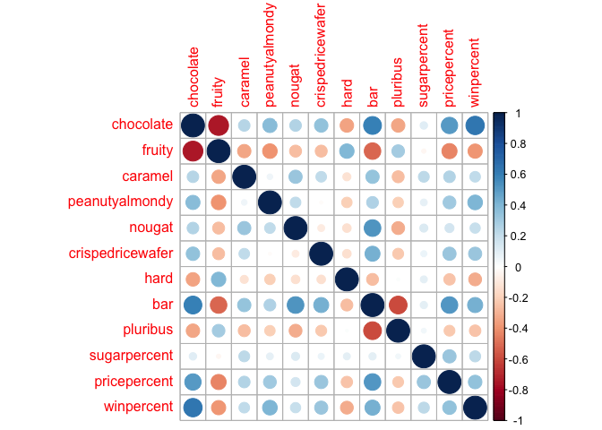
Q22. Examining this plot what two variables are anti-correlated (i.e. have minus values)?
Chocolate and fruity
Q23. Similarly, what two variables are most positively correlated?
Chocolate and winpercent.
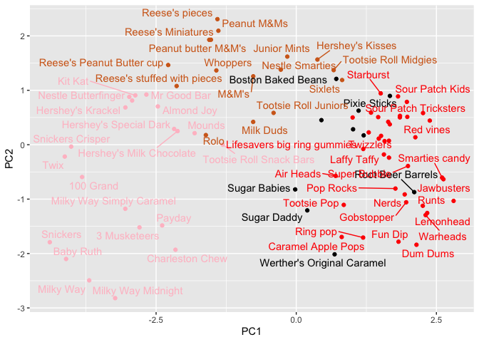
Principal Component Analysis
The function to use is called prcomp() with an optional scale=T/F
argument.
pca <- prcomp(candy, scale = TRUE)
summary(pca)
Importance of components:
                          PC1    PC2    PC3     PC4    PC5     PC6     PC7
Standard deviation     2.0788 1.1378 1.1092 1.07533 0.9518 0.81923 0.81530
Proportion of Variance 0.3601 0.1079 0.1025 0.09636 0.0755 0.05593 0.05539
Cumulative Proportion  0.3601 0.4680 0.5705 0.66688 0.7424 0.79830 0.85369
                           PC8     PC9    PC10    PC11    PC12
Standard deviation     0.74530 0.67824 0.62349 0.43974 0.39760
Proportion of Variance 0.04629 0.03833 0.03239 0.01611 0.01317
Cumulative Proportion  0.89998 0.93832 0.97071 0.98683 1.00000
Our main PCA result figure
ggplot(pca$x) +
  aes(PC1, PC2, label = rownames(pca$x)) +
  geom_point(col=my_cols) +
  geom_text_repel(col = my_cols)
Warning: ggrepel: 21 unlabeled data points (too many overlaps). Consider
increasing max.overlaps
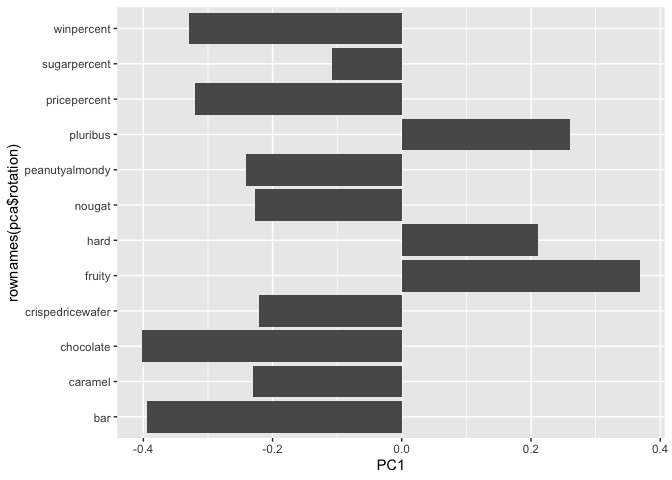
We should also examine the variable “loadings” or contributions of the origional variables to the new PCs
ggplot(pca$rotation) +
  aes(PC1, rownames(pca$rotation)) +
  geom_col()
p <- ggplot(pca$x) +
  aes(PC1, PC2, label = rownames(pca$x)) +
  geom_point(col=my_cols) +
  geom_text_repel(col = my_cols)
Interactive plots that can be zoomed on and “brushed” over can be made with the plotly package. it’s output is inter5active and willl not render to PDF :-(
library(plotly)
Attaching package: 'plotly'

The following object is masked from 'package:ggplot2':

    last_plot

The following object is masked from 'package:stats':

    filter

The following object is masked from 'package:graphics':

    layout
#plotly(p)
Q24. What original variables are picked up strongly by PC1 in the positive direction? Do these make sense to you?
Fruity, hard, pluribus. Yes, that makes sense: PC1 seems to capture a “non-chocolate, hard, multi-piece/fruit-flavor” axis, contrasting those candies with chocolate/bar/nutty/nougat types that load negatively.