Blinda's Class
Classwork for BIMM143
Lab 14 RNASeq mini project
Blinda Sui (PID: A17117043)
Background
Here we work through a complete RNASeq analysis project. The input data comes from a knock-down experiment of a HOX genes
Data Import
Reading the counts and metadata CSV files
counts <- read.csv("GSE37704_featurecounts.csv", row.names = 1)
metadata <- read.csv("GSE37704_metadata.csv")
Check on data structure
head(counts)
                length SRR493366 SRR493367 SRR493368 SRR493369 SRR493370
ENSG00000186092    918         0         0         0         0         0
ENSG00000279928    718         0         0         0         0         0
ENSG00000279457   1982        23        28        29        29        28
ENSG00000278566    939         0         0         0         0         0
ENSG00000273547    939         0         0         0         0         0
ENSG00000187634   3214       124       123       205       207       212
                SRR493371
ENSG00000186092         0
ENSG00000279928         0
ENSG00000279457        46
ENSG00000278566         0
ENSG00000273547         0
ENSG00000187634       258
metadata
         id     condition
1 SRR493366 control_sirna
2 SRR493367 control_sirna
3 SRR493368 control_sirna
4 SRR493369      hoxa1_kd
5 SRR493370      hoxa1_kd
6 SRR493371      hoxa1_kd
Some book-keeping is required as there looks to be a mis-match between metadata rows and counts columns
ncol(counts)
[1] 7
nrow(metadata)
[1] 6
Looks like we need to get rid of the first “length” column of our
counts object
Q. Complete the code below to remove the troublesome first column from countData
cleancounts <- counts[,-1]
colnames(cleancounts)
[1] "SRR493366" "SRR493367" "SRR493368" "SRR493369" "SRR493370" "SRR493371"
metadata$id
[1] "SRR493366" "SRR493367" "SRR493368" "SRR493369" "SRR493370" "SRR493371"
all(colnames(cleancounts) == metadata$id)
[1] TRUE
Remove zero count genes
There are lots of genes with zero counts. We can remove these from further analysis.
head(cleancounts)
                SRR493366 SRR493367 SRR493368 SRR493369 SRR493370 SRR493371
ENSG00000186092         0         0         0         0         0         0
ENSG00000279928         0         0         0         0         0         0
ENSG00000279457        23        28        29        29        28        46
ENSG00000278566         0         0         0         0         0         0
ENSG00000273547         0         0         0         0         0         0
ENSG00000187634       124       123       205       207       212       258
Q. Complete the code below to filter countData to exclude genes (i.e. rows) where we have 0 read count across all samples (i.e. columns).
to.keep.inds <- rowSums(cleancounts) > 0
nonzero_counts <- cleancounts[to.keep.inds,]
DESeq analysis
Load the package
library(DESeq2)
Setup DESeq
dds <- DESeqDataSetFromMatrix(countData = nonzero_counts,
                              colData = metadata,
                              design = ~condition)
Warning in DESeqDataSet(se, design = design, ignoreRank): some variables in
design formula are characters, converting to factors
Run DESeq
dds <- DESeq(dds)
estimating size factors

estimating dispersions

gene-wise dispersion estimates

mean-dispersion relationship

final dispersion estimates

fitting model and testing
Get results
res <- results(dds)
Q. Call the summary() function on your results to get a sense of how many genes are up or down-regulated at the default 0.1 p-value cutoff.
summary(res)
out of 15975 with nonzero total read count
adjusted p-value < 0.1
LFC > 0 (up)       : 4349, 27%
LFC < 0 (down)     : 4396, 28%
outliers [1]       : 0, 0%
low counts [2]     : 1237, 7.7%
(mean count < 0)
[1] see 'cooksCutoff' argument of ?results
[2] see 'independentFiltering' argument of ?results
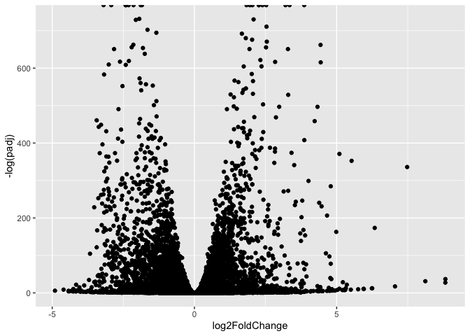
Data Visualization
Volcano plot
library(ggplot2)

ggplot(res) +
  aes(log2FoldChange, -log(padj)) +
  geom_point()
Warning: Removed 1237 rows containing missing values or values outside the scale range
(`geom_point()`).
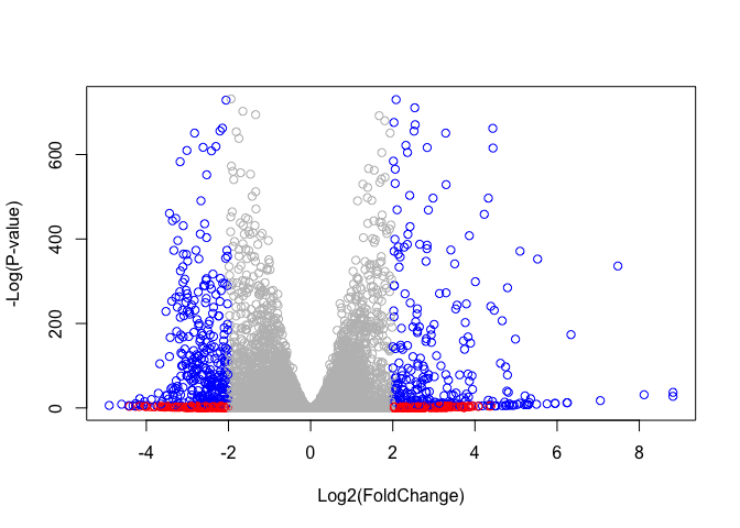
Q. Improve this plot by completing the below code, which adds color and axis labels
# Make a color vector for all genes
mycols <- rep("gray", nrow(res) )

# Color red the genes with absolute fold change above 2
mycols[ abs(res$log2FoldChange) > 2 ] <- "red"

# Color blue those with adjusted p-value less than 0.01
# and absolute fold change more than 2
inds <- (res$padj < 0.01) & (abs(res$log2FoldChange) > 2)
mycols[ inds ] <- "blue"

plot( res$log2FoldChange, -log(res$padj),
      col = mycols,
      xlab = "Log2(FoldChange)", ylab = "-Log(P-value)" )
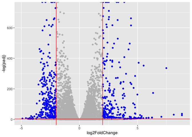
Add threshold lines for fold-change and P-value and color our subset of genes that make these threshold cut-offs in the plot
mycols <- rep("gray", nrow(res))
mycols[abs(res$log2FoldChange) > 2 & res$padj < 0.05] <- "blue"

ggplot(res) +
  aes(log2FoldChange, -log(padj), color = mycols) +
  geom_point() +
  geom_vline(xintercept = c(-2, 2), color = "red") +
  geom_hline(yintercept = -log(0.05), color = "red") +
  scale_color_identity()
Warning: Removed 1237 rows containing missing values or values outside the scale range
(`geom_point()`).
Add Annotation
Q. Use the mapIDs() function multiple times to add SYMBOL, ENTREZID and GENENAME annotation to our results by completing the code below.
Add some symbols and entrez ids
library(AnnotationDbi)
library(org.Hs.eg.db)
columns(org.Hs.eg.db)
 [1] "ACCNUM"       "ALIAS"        "ENSEMBL"      "ENSEMBLPROT"  "ENSEMBLTRANS"
 [6] "ENTREZID"     "ENZYME"       "EVIDENCE"     "EVIDENCEALL"  "GENENAME"
[11] "GENETYPE"     "GO"           "GOALL"        "IPI"          "MAP"
[16] "OMIM"         "ONTOLOGY"     "ONTOLOGYALL"  "PATH"         "PFAM"
[21] "PMID"         "PROSITE"      "REFSEQ"       "SYMBOL"       "UCSCKG"
[26] "UNIPROT"
res$symbol <- mapIds(x = org.Hs.eg.db,
                     keys = row.names(res),
                     keytype = "ENSEMBL",
                     column = "SYMBOL")
'select()' returned 1:many mapping between keys and columns
res$entrez <- mapIds(x = org.Hs.eg.db,
                     keys = row.names(res),
                     keytype = "ENSEMBL",
                     column = "ENTREZID")
'select()' returned 1:many mapping between keys and columns
res$name <- mapIds(x = org.Hs.eg.db,
                     keys = row.names(res),
                     keytype = "ENSEMBL",
                     column = "GENENAME")
'select()' returned 1:many mapping between keys and columns
Q. Finally for this section let’s reorder these results by adjusted p-value and save them to a CSV file in your current project directory.
res = res[order(res$padj), ]
write.csv(res, file = "deseq_results.csv")
Pathway Analysis
Run gene analysis
library(gage)
library(gageData)
library(pathview)
We need a named vector of fold-change values as input for gage
foldchanges <- res$log2FoldChange
names(foldchanges) <- res$entrez
head(foldchanges)
     1266     54855      1465      2034      2150      6659
-2.422719  3.201955 -2.313738 -1.888019  3.344508  2.392288
data("kegg.sets.hs")

keggres = gage(foldchanges, gsets=kegg.sets.hs)
attributes(keggres)
$names
[1] "greater" "less"    "stats"
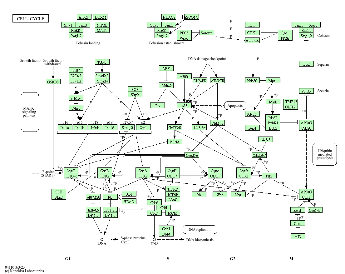
head(keggres$less, 5)
p.geomean stat.mean
hsa04110 Cell cycle 8.995727e-06 -4.378644
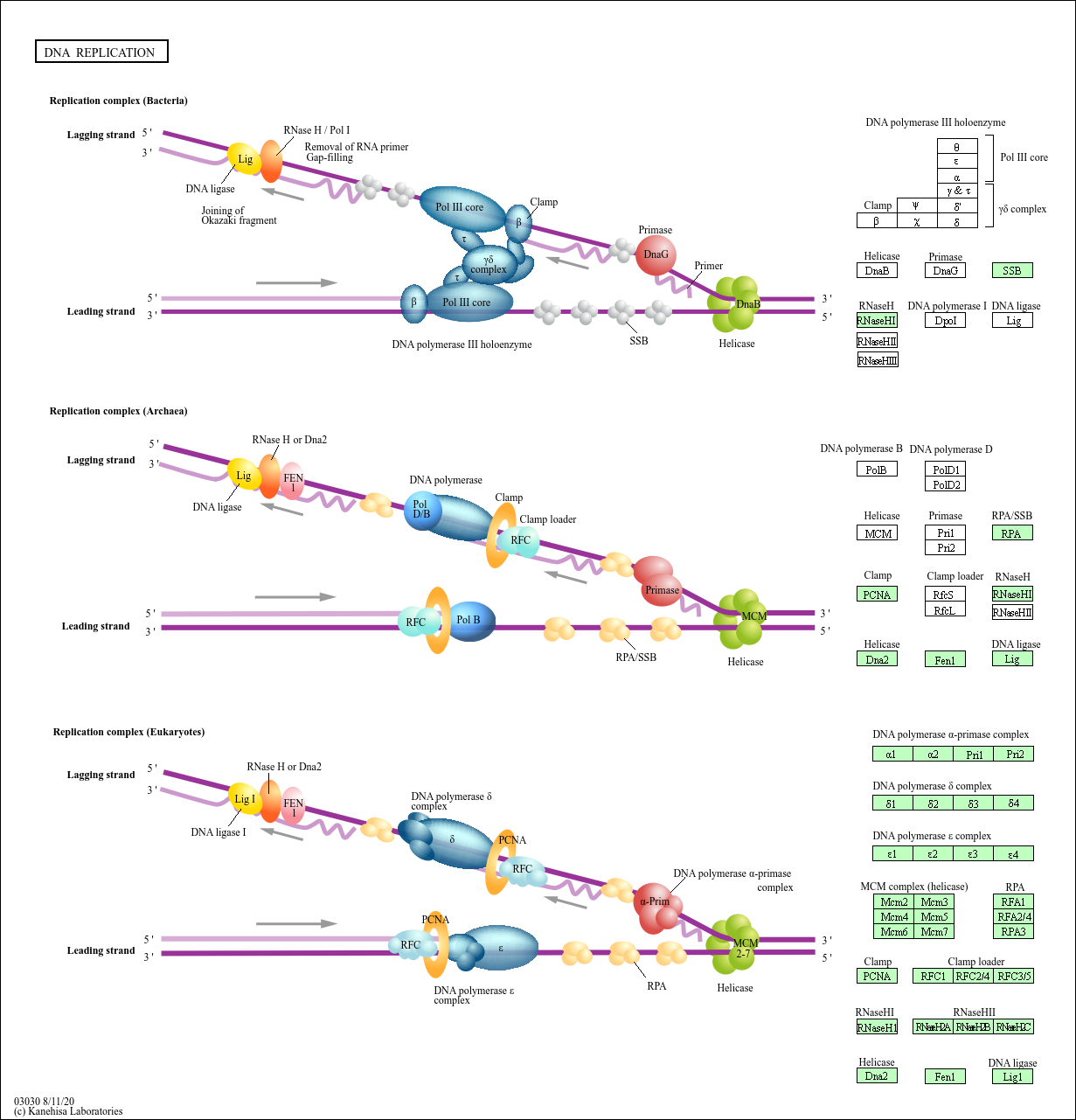
hsa03030 DNA replication 9.424076e-05 -3.951803
hsa05130 Pathogenic Escherichia coli infection 1.405864e-04 -3.765330
hsa03013 RNA transport 1.375901e-03 -3.028500
hsa03440 Homologous recombination 3.066756e-03 -2.852899
p.val q.val
hsa04110 Cell cycle 8.995727e-06 0.001889103
hsa03030 DNA replication 9.424076e-05 0.009841047
hsa05130 Pathogenic Escherichia coli infection 1.405864e-04 0.009841047
hsa03013 RNA transport 1.375901e-03 0.072234819
hsa03440 Homologous recombination 3.066756e-03 0.128803765
set.size exp1
hsa04110 Cell cycle 121 8.995727e-06
hsa03030 DNA replication 36 9.424076e-05
hsa05130 Pathogenic Escherichia coli infection 53 1.405864e-04
hsa03013 RNA transport 144 1.375901e-03
hsa03440 Homologous recombination 28 3.066756e-03
pathview(pathway.id="hsa04110", gene.data=foldchanges)
'select()' returned 1:1 mapping between keys and columns

Info: Working in directory /Users/blindasui/Desktop/BIMM143_bioinformatics/bimm143_github/Lab14

Info: Writing image file hsa04110.pathview.png
pathview(pathway.id = "hsa03030", gene.data = foldchanges)
'select()' returned 1:1 mapping between keys and columns

Info: Working in directory /Users/blindasui/Desktop/BIMM143_bioinformatics/bimm143_github/Lab14

Info: Writing image file hsa03030.pathview.png
 ### Gene Ontology (GO) Same analysis but using GO
genesets rather than KEGG
### Gene Ontology (GO) Same analysis but using GO
genesets rather than KEGG
data(go.sets.hs)
data(go.subs.hs)

# Focus on Biological Process subset of GO
gobpsets = go.sets.hs[go.subs.hs$BP]

gobpres = gage(foldchanges, gsets=gobpsets, same.dir=TRUE)

lapply(gobpres, head)
$greater
                                             p.geomean stat.mean        p.val
GO:0007156 homophilic cell adhesion       8.519724e-05  3.824205 8.519724e-05
GO:0002009 morphogenesis of an epithelium 1.396681e-04  3.653886 1.396681e-04
GO:0048729 tissue morphogenesis           1.432451e-04  3.643242 1.432451e-04
GO:0007610 behavior                       1.925222e-04  3.565432 1.925222e-04
GO:0060562 epithelial tube morphogenesis  5.932837e-04  3.261376 5.932837e-04
GO:0035295 tube development               5.953254e-04  3.253665 5.953254e-04
                                              q.val set.size         exp1
GO:0007156 homophilic cell adhesion       0.1951953      113 8.519724e-05
GO:0002009 morphogenesis of an epithelium 0.1951953      339 1.396681e-04
GO:0048729 tissue morphogenesis           0.1951953      424 1.432451e-04
GO:0007610 behavior                       0.1967577      426 1.925222e-04
GO:0060562 epithelial tube morphogenesis  0.3565320      257 5.932837e-04
GO:0035295 tube development               0.3565320      391 5.953254e-04

$less
                                            p.geomean stat.mean        p.val
GO:0048285 organelle fission             1.536227e-15 -8.063910 1.536227e-15
GO:0000280 nuclear division              4.286961e-15 -7.939217 4.286961e-15
GO:0007067 mitosis                       4.286961e-15 -7.939217 4.286961e-15
GO:0000087 M phase of mitotic cell cycle 1.169934e-14 -7.797496 1.169934e-14
GO:0007059 chromosome segregation        2.028624e-11 -6.878340 2.028624e-11
GO:0000236 mitotic prometaphase          1.729553e-10 -6.695966 1.729553e-10
                                                q.val set.size         exp1
GO:0048285 organelle fission             5.841698e-12      376 1.536227e-15
GO:0000280 nuclear division              5.841698e-12      352 4.286961e-15
GO:0007067 mitosis                       5.841698e-12      352 4.286961e-15
GO:0000087 M phase of mitotic cell cycle 1.195672e-11      362 1.169934e-14
GO:0007059 chromosome segregation        1.658603e-08      142 2.028624e-11
GO:0000236 mitotic prometaphase          1.178402e-07       84 1.729553e-10

$stats
                                          stat.mean     exp1
GO:0007156 homophilic cell adhesion        3.824205 3.824205
GO:0002009 morphogenesis of an epithelium  3.653886 3.653886
GO:0048729 tissue morphogenesis            3.643242 3.643242
GO:0007610 behavior                        3.565432 3.565432
GO:0060562 epithelial tube morphogenesis   3.261376 3.261376
GO:0035295 tube development                3.253665 3.253665
head(gobpres$less, 4)
                                            p.geomean stat.mean        p.val
GO:0048285 organelle fission             1.536227e-15 -8.063910 1.536227e-15
GO:0000280 nuclear division              4.286961e-15 -7.939217 4.286961e-15
GO:0007067 mitosis                       4.286961e-15 -7.939217 4.286961e-15
GO:0000087 M phase of mitotic cell cycle 1.169934e-14 -7.797496 1.169934e-14
                                                q.val set.size         exp1
GO:0048285 organelle fission             5.841698e-12      376 1.536227e-15
GO:0000280 nuclear division              5.841698e-12      352 4.286961e-15
GO:0007067 mitosis                       5.841698e-12      352 4.286961e-15
GO:0000087 M phase of mitotic cell cycle 1.195672e-11      362 1.169934e-14
Reactome
Lots of folks like the reactome web interface,. You can also run this as an R funciton but lets look at the website first. < https://reactome.org/ >
The website wants a text file wit one gene symbol per line of the genes you want to map to pathways.
sig_genes <- res[res$padj <= 0.05 & !is.na(res$padj), ]$symbol
head(sig_genes) #res$symbo
ENSG00000117519 ENSG00000183508 ENSG00000159176 ENSG00000116016 ENSG00000164251
         "CNN3"        "TENT5C"         "CSRP1"         "EPAS1"         "F2RL1"
ENSG00000124766
         "SOX4"
and write out to a file”
write.table(sig_genes, file="significant_genes.txt", row.names=FALSE, col.names=FALSE, quote=FALSE)
Save Our Results
write.csv(res, file="myresults.csv")
Q. Can you do the same procedure as above to plot the pathview figures for the top 5 down-reguled pathways?
## Focus on top 5 downregulated pathways
keggrespathways_down <- rownames(keggres$less)[1:5]

# Extract the 8-character KEGG IDs
keggresids_down <- substr(keggrespathways_down, start = 1, stop = 8)

# Draw pathview plots for these pathways
pathview(gene.data = foldchanges,
         pathway.id = keggresids_down,
         species = "hsa")
'select()' returned 1:1 mapping between keys and columns

Info: Working in directory /Users/blindasui/Desktop/BIMM143_bioinformatics/bimm143_github/Lab14

Info: Writing image file hsa04110.pathview.png

'select()' returned 1:1 mapping between keys and columns

Info: Working in directory /Users/blindasui/Desktop/BIMM143_bioinformatics/bimm143_github/Lab14

Info: Writing image file hsa03030.pathview.png

'select()' returned 1:1 mapping between keys and columns

Info: Working in directory /Users/blindasui/Desktop/BIMM143_bioinformatics/bimm143_github/Lab14

Info: Writing image file hsa05130.pathview.png

'select()' returned 1:1 mapping between keys and columns

Info: Working in directory /Users/blindasui/Desktop/BIMM143_bioinformatics/bimm143_github/Lab14

Info: Writing image file hsa03013.pathview.png

'select()' returned 1:1 mapping between keys and columns

Info: Working in directory /Users/blindasui/Desktop/BIMM143_bioinformatics/bimm143_github/Lab14

Info: Writing image file hsa03440.pathview.png
Q: What pathway has the most significant “Entities p-value”? Do the most significant pathways listed match your previous KEGG results? What factors could cause differences between the two methods?
In Reactome, the most significant pathway by Entities p-value was ‘[Reactome top pathway]’, which is involved in cell cycle control. This agrees well with our KEGG gage results, where the most strongly enriched pathway was Cell cycle (hsa04110), along with other DNA replication and mitosis-related pathways. Any differences between the Reactome and KEGG results likely arise from differences in how the two databases define pathways (Reactome has more granular pathway splits), differences in the underlying gene sets and background universe, the specific statistical tests and multiple-testing corrections used, and small discrepancies in gene ID mapping and the significance thresholds we chose.
Q: What pathway has the most significant “Entities p-value”? Do the most significant pathways listed match your previous KEGG results? What factors could cause differences between the two methods?
The online GO enrichment analysis (Biological Process, Homo sapiens) reported ‘[top GO BP term]’ as the most significantly enriched term. This process is directly related to cell cycle regulation and mitosis, consistent with our KEGG and Reactome results, which also highlighted cell cycle pathways as strongly perturbed. Differences in the exact top terms between GO, KEGG, and Reactome are expected because these resources define gene sets differently, use distinct statistical enrichment methods and background gene universes, and sometimes differ in gene ID mappings and annotation granularity.